10 Advanced SQL Concepts You Should Know for Data Science Interviews
- Common table expressions (CTEs).
- Recursive CTEs.
- Temporary functions.
- Pivoting data with case when.
- Except versus Not In.
- Self joins.
- Rank versus dense rank versus row number.
- Calculating delta values.
- Calculating running totals.
- Date-time manipulation.
1. Common Table Expressions (CTEs)
If you’ve ever wanted to query a query, that’s when common table expressions (CTEs) come into play. CTEs essentially create a temporary table.
Using CTEs is a great way to modularize and break down your code just like you would break an essay down into several paragraphs.
Consider the following query with a subquery in the where clause:
SELECT name
       , salary
FROM People
WHERE name in (SELECT DISTINCT name
               FROM population
               WHERE country = "Canada"
                     AND city = "Toronto")
      AND salary >= (SELECT AVG(salary)
                     FROM salaries
                     WHERE gender = "Female")
This may not seem too difficult to understand, but what if there were many subqueries or subqueries within subqueries? This is where CTEs come into play.
with toronto_ppl as (
   SELECT DISTINCT name
   FROM population
   WHERE country = "Canada"
         AND city = "Toronto"
)
, avg_female_salary as (
   SELECT AVG(salary) as avgSalary
   FROM salaries
   WHERE gender = "Female"
)
SELECT name
       , salary
FROM People
WHERE name in (SELECT DISTINCT FROM toronto_ppl)
      AND salary >= (SELECT avgSalary FROM avg_female_salary)
Now, the where clause is clearly filtering for names in Toronto. CTEs are useful both because you can break down your code into smaller chunks and because you can assign a variable name to each CTE (i.e., toronto_ppl and avg_female_salary).
CTEs also allow you to do more advanced techniques like creating recursive tables.
2. Recursive CTEs
A recursive CTE is a CTE that references itself, just like a recursive function in Python. Recursive CTEs are especially useful when querying hierarchical data like organization charts, file systems, a graph of links between web pages, and so on.
A recursive CTE has three parts:
- The anchor member, which is an initial query that returns the base result of the CTE.
- The recursive member is a recursive query that references the CTE. This is
UNION ALLed with the anchor member - A termination condition that stops the recursive member.
Here’s an example of a recursive CTE that gets the manager ID for each staff ID:
with org_structure as (
   SELECT id
          , manager_id
   FROM staff_members
   WHERE manager_id IS NULL
   UNION ALL
   SELECT sm.id
          , sm.manager_id
   FROM staff_members sm
   INNER JOIN org_structure os
      ON os.id = sm.manager_id
3. Temporary Functions
Knowing how to write temporary functions is important for several reasons:
- It allows you to break code down into smaller chunks.
- It’s useful for writing cleaner code.
- It prevents repetition and allows you to reuse code, similar to using functions in Python.
Consider the following example:
SELECT name
       , CASE WHEN tenure < 1 THEN "analyst"
              WHEN tenure BETWEEN 1 and 3 THEN "associate"
              WHEN tenure BETWEEN 3 and 5 THEN "senior"
              WHEN tenure > 5 THEN "vp"
              ELSE "n/a"
         END AS seniority
FROM employees
Instead, you can leverage a temporary function to capture the CASE clause.
CREATE TEMPORARY FUNCTION get_seniority(tenure INT64) AS (
   CASE WHEN tenure < 1 THEN "analyst"
        WHEN tenure BETWEEN 1 and 3 THEN "associate"
        WHEN tenure BETWEEN 3 and 5 THEN "senior"
        WHEN tenure > 5 THEN "vp"
        ELSE "n/a"
   END
);
SELECT name
       , get_seniority(tenure) as seniority
FROM employees
With a temporary function, the query itself is much simpler and more readable. You can also reuse the seniority function. For more on temporary functions,
4. Pivoting Data With Case When
You’ll most likely see many questions that require the use of case when statements, and that’s simply because it’s such a versatile concept. It allows you to write complex conditional statements if you want to allocate a certain value or class depending on other variables.
Less commonly known, however, is that it also allows you to pivot data. For example, if you have a month column, and you want to create an individual column for each month, you can use case when statements to pivot the data.
Example Question: Write an SQL query to reformat the table so that there is a revenue column for each month.
Initial table:
+------+---------+-------+
| id   | revenue | month |
+------+---------+-------+
| 1    | 8000    | Jan   |
| 2    | 9000    | Jan   |
| 3    | 10000   | Feb   |
| 1    | 7000    | Feb   |
| 1    | 6000    | Mar   |
+------+---------+-------+
Result table:
+------+-------------+-------------+-------------+-----+-----------+
| id   | Jan_Revenue | Feb_Revenue | Mar_Revenue | ... | Dec_Revenue |
+------+-------------+-------------+-------------+-----+-----------+
| 1    | 8000        | 7000        | 6000        | ... | null        |
| 2    | 9000        | null        | null        | ... | null        |
| 3    | null        | 10000       | null        | ... | null        |
+------+-------------+-------------+-------------+-----+-----------+
5. Except vs Not In
Except and not in operate almost identically. They’re both used to compare the rows between two queries/tables. That being said, there are subtle nuances between the two that you should know.
First, except filters out duplicates and returns distinct rows, unlike not in.
Further, except expects the same number of columns in both queries/tables, whereas not in compares a single column from each query/table.
6. Self Joins
An SQL self-join joins a table with itself. You might think that such an action serves no purpose, but you’d be surprised at how common this is. In many real-life settings, data is stored in one large table rather than many smaller tables. In such cases, self-joins may be required to solve unique problems.
Let’s look at an example.
Example Question: Given the Employee table below, write a SQL query that finds employees who earn more than their managers.
+----+-------+--------+-----------+
| Id | Name  | Salary | ManagerId |
+----+-------+--------+-----------+
| 1  | Joe   | 70000  | 3         |
| 2  | Henry | 80000  | 4         |
| 3  | Sam   | 60000  | NULL      |
| 4  | Max   | 90000  | NULL      |
+----+-------+--------+-----------+
Answer:
SELECT
    a.Name as Employee
FROM
    Employee as a
    JOIN Employee as b on a.ManagerID = b.Id
WHERE a.Salary > b.Salary
For the above table, Joe is the only employee who earns more than his manager.
7. Rank vs Dense Rank vs Row Number
Ranking rows and values is a common application. Here are a few examples in which companies frequently use ranking:
- Ranking highest valued customers by number of purchases, profits, and so on.
- Ranking the top products sold by number of units sold.
- Ranking the top countries with the most sales.
- Ranking the top videos viewed by number of minutes watched, number of distinct viewers, and so on.
In SQL, there are several ways that you can assign a rank to a row, which we’ll dive into with an example. Consider the following query and results:
SELECT Name
       , GPA
       , ROW_NUMBER() OVER (ORDER BY GPA desc)
       , RANK() OVER (ORDER BY GPA desc)
       , DENSE_RANK() OVER (ORDER BY GPA desc)
FROM student_grades
ROW_NUMBER()returns a unique number for each row starting at one. When there are ties (e.g., Bob versus Carrie), ROW_NUMBER() arbitrarily assigns a number if a second criterion is not defined.
RANK()returns a unique number for each row starting at one, except for when there are ties, then RANK() will assign the same number. A gap will follow a duplicate rank.
DENSE_RANK()is similar to RANK() except that there are no gaps after a duplicate rank. Notice that with DENSE_RANK(), Daniel is ranked third as opposed to fourth with RANK().
8. Calculating Delta Values
Another common application is comparing values from different periods. For example, what was the delta between this month and last month’s sales? Or what was the delta between this month and the same one last year?
When comparing values from different periods to calculate deltas, this is when LEAD() and LAG() come into play.
Here are some examples:
# Comparing each month's sales to last month
SELECT month
       , sales
       , sales - LAG(sales, 1) OVER (ORDER BY month)
FROM monthly_sales
# Comparing each month's sales to the same month last year
SELECT month
       , sales
       , sales - LAG(sales, 12) OVER (ORDER BY month)
FROM monthly_sales
9. Calculating Running Totals
If you knew about ROW_NUMBER() and LAG()/LEAD(), this probably won’t be much of a surprise to you. But if you didn’t, this is probably one of the most useful window functions, especially when you want to visualize growth.
Using a window function with SUM(), we can calculate a running total. See the example below:
SELECT Month
       , Revenue
       , SUM(Revenue) OVER (ORDER BY Month) AS Cumulative
FROM monthly_revenue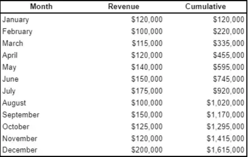
10. Date-Time Manipulation
You should definitely expect some sort of SQL questions that involve date-time data. For example, you may be required to group data by months or convert a variable format from DD-MM-YYYY to simply the month.
Some functions you should know are the following:
EXTRACTDATEDIFFDATE_ADD,DATE_SUBDATE_TRUNC
Example Question: Given a Weather table, write a SQL query to find all date IDs with higher temperatures compared to previous dates.
+---------+------------------+------------------+
| Id(INT) | RecordDate(DATE) | Temperature(INT) |
+---------+------------------+------------------+
|       1 |       2015-01-01 |               10 |
|       2 |       2015-01-02 |               25 |
|       3 |       2015-01-03 |               20 |
|       4 |       2015-01-04 |               30 |
+---------+------------------+------------------+
Answer:
SELECT
    a.Id
FROM
    Weather a,
    Weather b
WHERE
    a.Temperature > b.Temperature
    AND DATEDIFF(a.RecordDate, b.RecordDate) = 1
